Potts Model Visualized

Inspired by The Illustrated Transformer, this post unpacks the symbols behind a Potts Model and visualizes how its parameters help us understand the evolution of protein sequence and structure.

Introduction

Proteins are linear chains of molecules known as amino acids. There are 20 commonly occurring amino acids represented by twenty letters of the English alphabet A-Z except for BJOUXZ. To account for insertions and deletions, we include an additional letter ‘-‘ representing an amino acid of length zero. These amino acids are chained together in a string, so a single protein chain can be described by a string of letters such as MNFPRATANCSLQPLD. Many proteins fold into 3-dimensional structures as shown below (the structures shown are interactive).

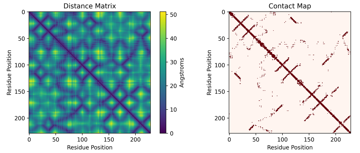
Such complicated twists and turns can be represented as a distance matrix, where entry row i and column j is the distance between residue i and residue j. Distance matrices can be binarized into a contact map where every entry in the matrix is either 0 or 1. If the entry in row i and column j of the contact map is 1, it represents that amino acid i is “in contact” with amino acid j. “In contact” usually means that the two amino acids are within some distance apart, usually 6 Angstroms. To get a sense of how small this is, it is about 1 millionth the width of a human hair. The distance matrix and contact map of protein 6EQD is shown below.

Evolutionary Constraints

A Potts model is a probabilistic model. For protein sequences, it is usually used to model a homologous set of sequences, i.e. sequences which likely evolved from one ancestral protein sequence. But what do we mean by “model”? A Potts model assigns each sequence a number which represents how likely that sequence belongs to this homologous set. Sequences in the homologous set are clearly likely to belong to the homologous set so they should be assigned high likelihoods. So why doesn’t the model just memorize all the homologous sequences, give them high likelihoods, and call it a day? We prevent this from happening by using a held-out set of sequences which the model does not see, and enforce the model to also have high likelihood on those sequences too. This simple setup allows Potts models to infer protein structure from sequence information alone. How?

First let’s try to reason about how the evolution of protein sequences work. The structural proximity of two amino acids can impose constraints on what mutations are allowable. For example, as shown in the figure below, we can see that certain amino acids are not allowed in the case of charged amino acids. This implies that by finding pairs of amino acids which evolve together (coevolve), rather than evolving independently, we can infer that these two positions are likely to be structurally adjacent. As an example, we can see the figure below which shows coevolution between the two blue positions.

Somehow the information of coevolving residues need to be captured in the Potts model. A Potts model does this by capturing the sitewise and pairwise frequencies in the sequence data. Sitewise means for some position i along the sequence, what are the probabilities of all the possible amino acids at that position. Pairwise means for some pair of positions i and j, what are the probabilities of all 21 by 21 pairs of amino acids in those two positions. It’s able to do this owing to an important concept in machine learning: inductive bias. The parameters of a Potts model directly correspond to the notion of capturing sitewise and pairwise frequencies, thus making them interpretable.

Potts Model Parameters

Now let’s take a look at the parameters of the model. The J parameter is a (L by 21) by (L by 21) matrix that looks like this:

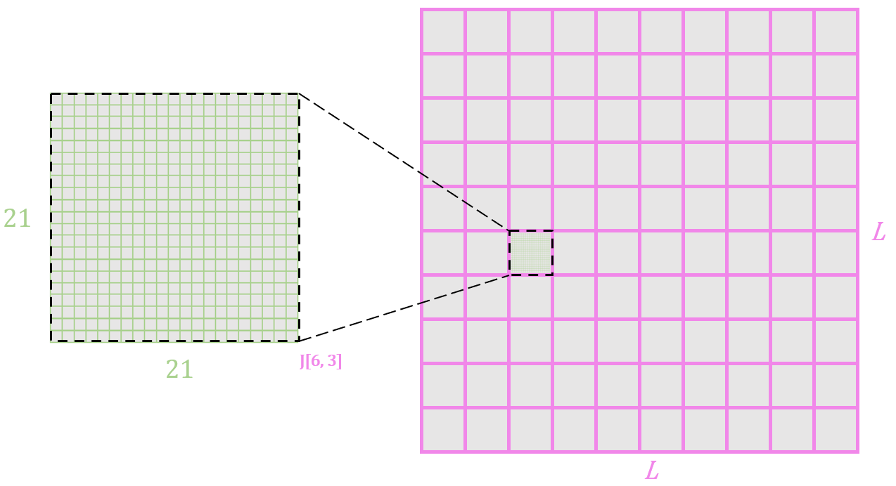
The 21x21 square shown models the pairwise frequencies of all possible 21x21 pairs of amino acids for amino acid positions 6 and 3. L = 10 in this example.

It also includes a parameter h which models the sitewise frequencies of sequences, looking like this:

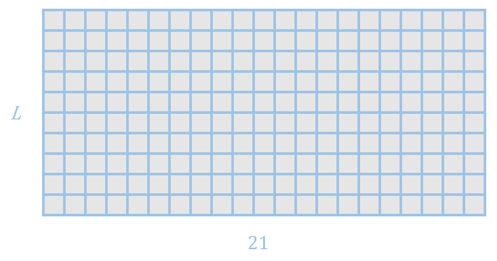
L = 10 in this example. For example, row 2 models the frequencies of the 21 amino acids (including gap) at position 2.

The input to a Potts model is a multiple sequence alignment. Conversion of a multiple sequence alignment to a numerical representation on the computer simply maps each amino acid to an integer between 0 and 20 inclusive. An example looks like this:

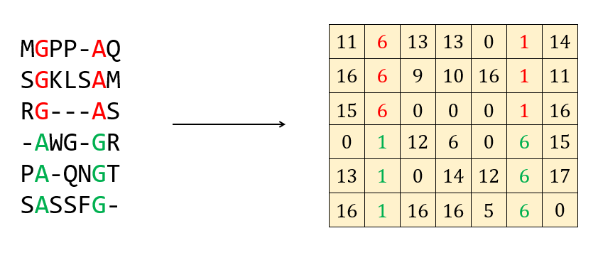
Here a pairwise correlation is shown in red and green. A Potts model should then predict these two positions as being in contact.

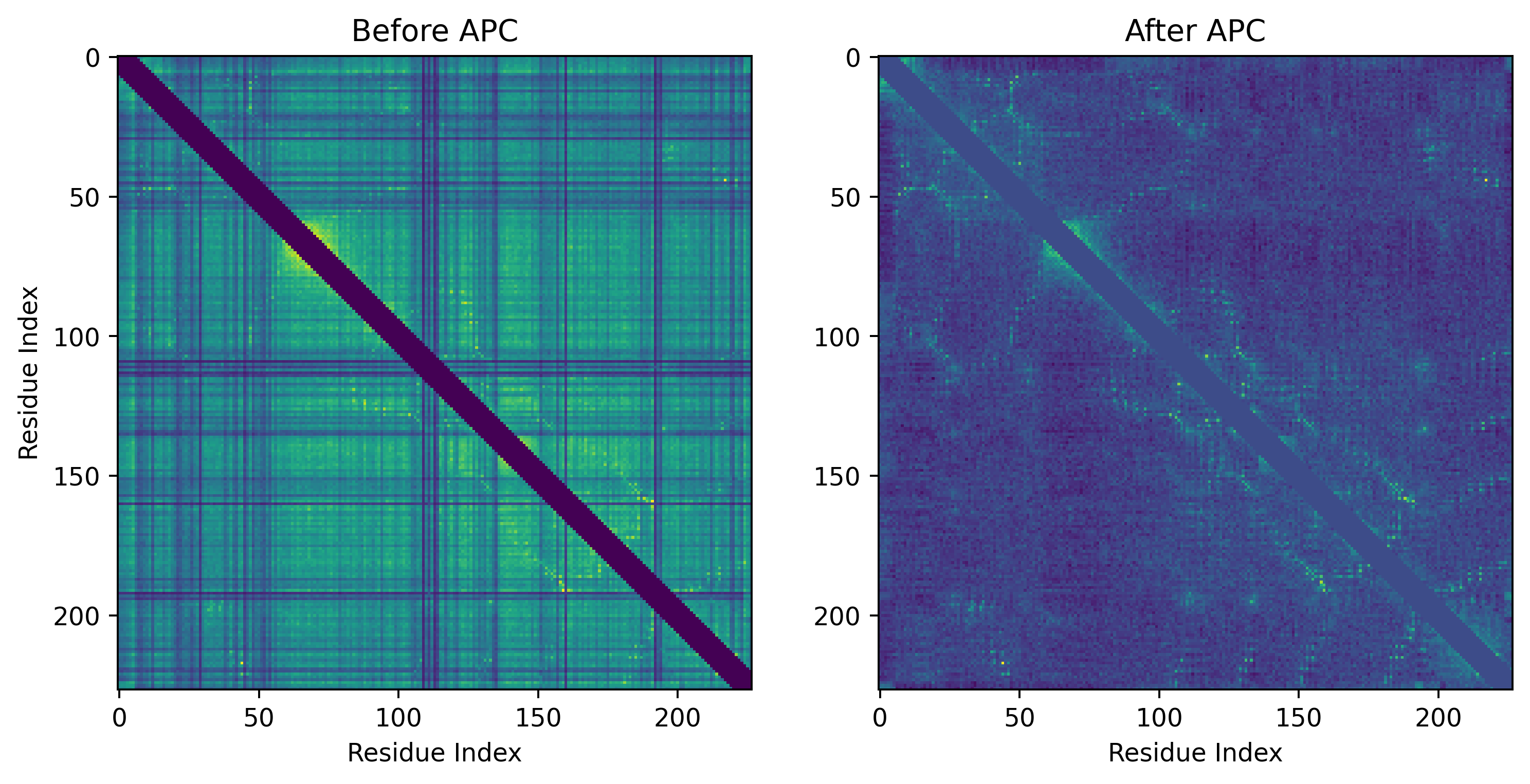
Notably, the J parameter captures pairwise correlations. However, just looking at the correlations between amino acid pairs is not enough. If A and B coevolve, but B and C also coevolve, this means A and C coevolve as well but they are not necessarily structurally adjacent. This phenomenon known as chaining needs to be disentangled from actual structurally adjacent pairs. To do this, we reduce the (L by 21) by (L by 21) matrix J into an L by L matrix by taking the sum of each 21 by 21 grid (green grid in the figure showing parameter J). Only after applying average product correction (APC) sifts out “direct couplings” from correlations from amino acids which show correlation but are not actually in contact. By only keeping the direct couplings, the patterns of protein contacts emerge.

We can visualize these predicted contacts on the structure of a protein in this homologous family. First let’s see the actual contacts:

Then let’s see the predicted contacts in black sticks:

An excellent PyTorch implementation of training such a model can be found here.

Various training strategies can be used to train a Potts model. As the final project, Syed Ather and I wrote a manuscript comparing how different training strategies affect modelling first/second order correlations, contact prediction, out-of-distribution detection, and correlation with the Rosetta Energy Function.

References

Balakrishnan, Sivaraman, et al. “Learning generative models for protein fold families.” Proteins: Structure, Function, and Bioinformatics 79.4 (2011): 1061-1078.

Ekeberg, Magnus, et al. “Improved contact prediction in proteins: using pseudolikelihoods to infer Potts models.” Physical Review E 87.1 (2013): 012707.